Biological Time Series - Marine Animals

4.3

Use of zooplankton communities to estimate the relative strength of the East Australian Current

Contributors

Wayne Rochester1

Frank Coman1

Claire Davies2

Ruth Eriksen2

Felicity McEnnulty2

Anita Slotwinski1

Marks Tonks1

Julian Uribe-Palomino1

Anthony J. Richardson1,3

1 CSIRO Oceans and Atmosphere, Queensland Biosciences Precinct (QBP), St Lucia, QLD, Australia
2 CSIRO Oceans and Atmosphere, Hobart, TAS, Australia
3 Centre for Applications in Natural Resource Mathematics (CARM), School of Mathematics and Physics, The University of Queensland, St Lucia, QLD, Australia

Key Information

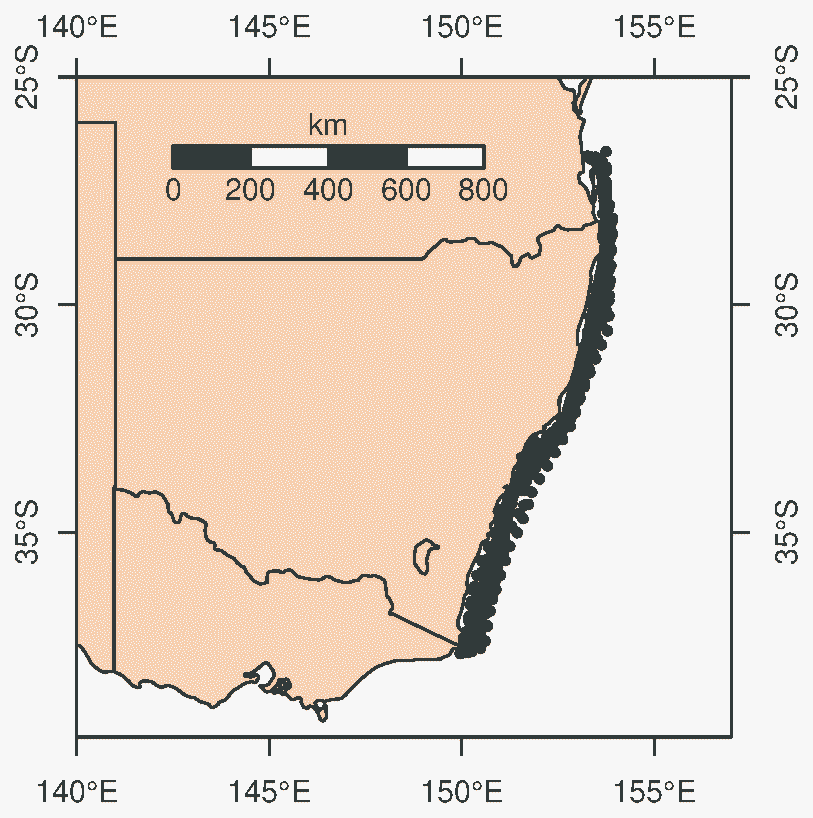
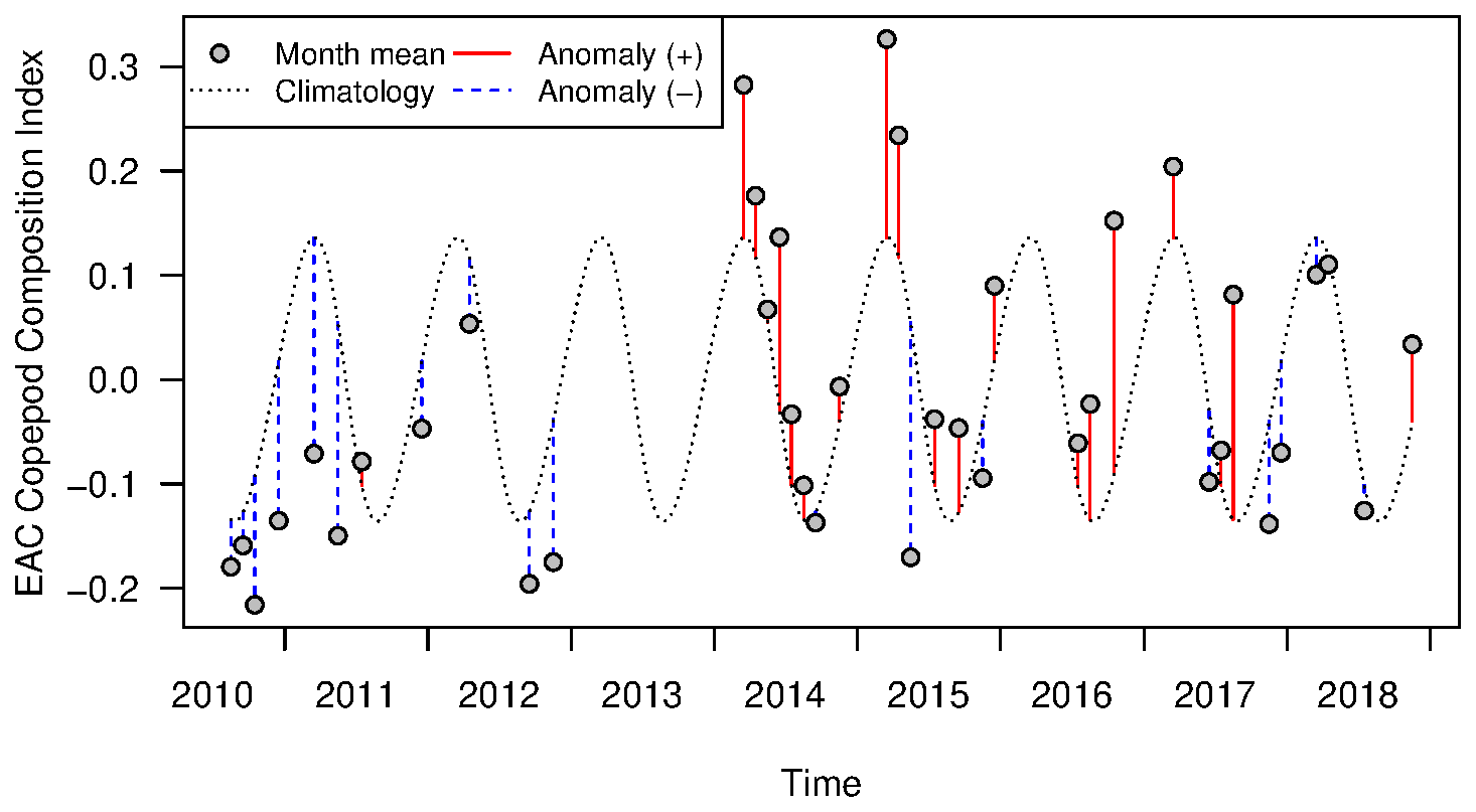
A time series of a water temperature index estimated from biological data alone was calculated from the semi-regular AusCPR transects of copepod species composition in the East Australian Current. This time series can potentially help detect changes in the EAC or monitor ecosystem responses to year-to-year variation and long-term trends in the physical and chemical environment, associated with EAC changes, ENSO and climate change.

Keywords

Climate change, Continuous Plankton Recorder, copepod composition index

Use of zooplankton communities to estimate the relative strength of the East Australian Current

The East Australian Current (EAC) is the major boundary current in Australia and transports warm water poleward along the east coast of Australia (K. Ridgway, Coleman, Bailey, & Sutton, 2008). In recent decades the EAC has extended further south, increasing the rate of warming in the Tasman Sea (K. R. Ridgway, 2007). The EAC has marked seasonality – its strength peaks in summer (February) and is weakest in winter (K. R. Ridgway & Godfrey, 1997). By transporting organisms from tropical to temperate Australia, the EAC is a major driver of the distribution of marine communities along the east coast of Australia (Poloczanska et al., 2007).

As zooplankton have short generation times and are not exploited, they are sensitive indicators of temperature and different water masses, especially copepods, the most abundant multicellular animals (Hays, Robinson, & Richardson, 2005). One might expect variation in copepod communities down the east coast of Australia, with warmer-water communities in the north and cooler-water ones in the south. More subtly, warmer-water communities could penetrate further south when the EAC is strongest. And we might also expect a signature of the interannual variation in the EAC – which has peaks and troughs about four years apart (K. Ridgway et al., 2008) – might be reflected in changes in the copepod community.

Here we explore whether long-term (2010-2018) changes in the copepod community along the east coast of Australia could be used as an index of the seasonal and inter-annual strength of the EAC. The Integrated Marine Observing System (IMOS) Australian Continuous Plankton Recorder (AusCPR) survey dataset is ideal for this because ships regularly traverse this route towing CPRs. If we can develop an index of the relative strength of the EAC along the CPR route down the east coast, then this could provide a large-scale metric independent of physical measurements and not estimated at a single cross-section across the current.

Copepod data were collected between Brisbane and the border between New South Wales and Victoria, a distance of ~1600 km (Figure 1). The AusCPR dataset comprised 766 samples (transect segments) from 56 trips from 2010 to 2018 and included 180 copepod species (https://portal.aodn.org.au/; see the dataset “IMOS - AusCPR: Zooplankton Abundance”). SST data were obtained from the IMOS Regional Australian Multi-Sensor SST Analysis dataset (Beggs et al., 2011); https://portal.aodn.org.au/; see the dataset “IMOS - SRS - SST - L4 - RAMSSA – Australia”).

We calculated a time series of an index of copepod species composition that was purposefully correlated with sea surface temperature (SST). We first conducted a multivariate redundancy analysis (RDA) of copepod species on SST, which ensures the multivariate index is maximally correlated with SST. We then used these sample scores from the multivariate RDA analysis as the univariate response in a generalised additive model, with latitude, day of year, and year as predictors (See Appendix for more details). Predictions from this model allowed us to produce a time series that reflects the copepod composition along the east coast of Australia. This time series included the seasonal, interannual and residual variation, but with the latitude effect removed. The anomalies and climatology can be plotted and interpreted analogously to, for example, the regional SST anomaly.

We have devised the EAC Copepod Composition Index to reflect changes in copepod communities down the east coast of Australia and thus to hopefully reproduce the relative strength of the EAC. If the index works, then the EAC should be stronger and the index more positive when warmer-water copepod communities are distributed further south. By contrast, the EAC should be weaker and the index more negative when warmer-water communities are confined to the north, and cooler-water communities dominate further south.

As expected, the EAC Copepod Composition Index anomaly is positively related to the general trends in the SST anomaly along the east coast from 2010-2018 (R=0.60, p<0.0001, n=39), showing that the index reflects changes in SST. The EAC Copepod Composition Index was driven by real changes in copepod communities: higher values of the Index equated to more warmer-water species such as Canthocalanus pauper, Temora turbinata and Centropages furcatus; and lower values equated to more cooler-water species such as Oncaea venusta, Acartia danae and Oncaea media (Figure 2).

The EAC Copepod Composition Index appears to reflect three characteristics of the EAC (Figure 3). The first is the Index has a strong seasonal cycle (the dotted line in Figure 3 is the climatology), with a peak in March and a trough in August, consistent with the known seasonality of the EAC (K. R. Ridgway & Godfrey, 1997) . The second characteristic is that deviations of the Index from the climatology are not random, but persist for extended periods (Figure 3). The anomalies indicate species compositions associated with cooler water from 2010-2012 (potentially weaker EAC flow), warmer water from 2014-2016 (potentially stronger EAC flow) and moderate water temperature from 2017-2018 (average EAC flow). From 1993-2006, K. Ridgway et al. (2008) found that the major interannual variation in strength of the EAC (peak-to-trough) was four years, similar to the three-year period we observed in the EAC Copepod Composition Index. Last, the Index is also weakly related to ENSO, with a stronger index under El Niño conditions (R=-0.38, p=0.02, n=39), similar to other studies that have shown similar weak relationship between EAC flow and ENSO (Holbrook, Chan, & Venegas, 2005).

It is difficult to measure the EAC strength along its whole extent, with most physical oceanographic methods estimating the flow over a cross section at a particular point. There are also breaks in the time series measurements. Developing an index based on biology could provide an independent along-EAC estimate of its strength, and potentially help to fill gaps in physical time series. Further, the EAC Copepod Composition Index tells us how the copepod community along the east coast is changing, providing a potentially valuable index for monitoring impacts of climate change. This could be especially valuable considering that the EAC is projected to continue increasing in strength in the future (Cai, Shi, Cowan, Bi, & Ribbe, 2005).

Regular transects by IMOS CPRs enable us to monitor changes in the offshore marine ecosystem that may be associated with year-to-year variation and long-term trends in the physical and chemical environment. These are potentially associated with changes in the EAC, ENSO and climate change. The next step is to further test the EAC Copepod Composition Index using model output (e.g., Bluelink) or measurements from the EAC array or proxy sources (e.g., XBT, CTD and satellite altimetry, Ridgway et al. (2008).

In the calculation of the EAC Copepod Composition Index, we used a distance-based RDA (db-RDA), which transforms the community matrix with a transformation (here the Hellinger transformation) that both works well with species data and retains the Euclidean properties that enable the standard RDA method to be applied. Use of the Hellinger transformation implies that the analysis considered species composition only (i.e. percentage of sample animals in each species) and not absolute abundance. The outcome of this approach is that the value of the RDA score for a sample is the weighted average of the (transformed) percent contribution of each species to the sample total, with the species weights calculated (by the RDA) to ensure the score is correlated with SST.

As for SST, copepod species composition is correlated with latitude and season (Figure 4). To calculate our final index and anomalies from the RDA score, we removed the latitude component and calculated a climatology. We termed the final index the EAC Copepod Composition Index. Because the CPR deployment times are seasonal but often irregular because of shipping schedules, these steps could not be performed using simple calculations based on monthly averages. Instead, we used the following generalised additive model (GAM):

y = a + fs(s) + fl(l) + ft(t) + e

where y is the RDA score, s is day of year, l is latitude, t is time (for trend across years), a is the intercept, e is the residual error and fs, fl and ft are GAM spline functions (with fs being cyclic). This model conveniently decomposed the RDA scores into components that we could combine by simple arithmetic to create the EAC Copepod Composition Index and climatology (Figure 5). We calculated the EAC Copepod Composition Index by subtracting the latitude component of the fitted values (i.e. y' = yfl(l)). The climatology was calculated as the sum of the day-of-year and intercept components of the GAM predicted values (i.e. yc = a + fs(s)). (Note that these calculations rely on fact that the GAM spline functions are constrained to sum to zero over the range of the data.) There is a clear climatology, with a stronger EAC copepod composition index during summer and weaker during winter (Figure 5). The latitudinal effect is nearly linear, but is steeper at more southern latitudes, implying the index is more sensitive to changes there than further north. The interannual time series shows there is longer-term persistent variation (Figure 5).

For plotting and further interpretation, the EAC Copepod Composition Index was aggregated to a monthly average. We then plot this output as the EAC Copepod Composition Index (Figure 3), and visualise it by including the climatology and anomalies from these.

Beggs, H., Aihong, Z., Graham, W., Oscar, A., Brassington, G., & Pugh, T. (2011). RAMSSA-An operational, high-resolution, Regional Australian Multi-Sensor Sea surface temperature Analysis over the Australian region (Vol. 61).

Cai, W., Shi, G., Cowan, T., Bi, D., & Ribbe, J. (2005). The response of the Southern Annular Mode, the East Australian Current, and the southern mid-latitude ocean circulation to global warming. Geophysical Research Letters, 32(23). doi:10.1029/2005gl024701

Hays, G. C., Robinson, C., & Richardson, A. J. (2005). Climate change and marine plankton. Trends in Ecology and Evolution, 20(6), 337-344.

Holbrook, N. J., Chan, P. S.-L., & Venegas, S. A. (2005). Oscillatory and propagating modes of temperature variability at the 3–3.5- and 4–4.5-yr time scales in the upper southwest Pacific Ocean. Journal of Climate, 18 (719-736), 1637–1639.

Poloczanska, E. S., Babcock, R. C., Butler, A., Hobday, A., Hoegh-Guldberg, O., Kunz, T. J., . . . Richardson, A. J. (2007). Climate change and Australian marine life. Oceanography and marine biology: an annual review, 45, 407-478. Retrieved from <Go to ISI>://WOS:000252476600008

Ridgway, K., Coleman, R., Bailey, R., & Sutton, P. (2008). Decadal variability of East Australian Current transport inferred from repeated high-density XBT transects, a CTD survey and satellite altimetry. 113. doi:10.1029/2007JC004664

Ridgway, K. R. (2007). Long-term trend and decadal variability of the southward penetration of the East Australian Current. Geophysical Research Letters, 34(13), 1-5. doi:L13613

10.1029/2007gl030393

Ridgway, K. R., & Godfrey, J. S. (1997). Seasonal cycle of the East Australian Current. Journal of Geophysical Research: Oceans, 102(C10), 22921-22936. doi:10.1029/97JC00227

Figure 1

Locations of the CPR samples used in the analysis (nominal locations of transect segments).

Figure 2

The temperature preferences of key species contributing to higher values of the EAC Copepod Composition Index (warm-water anomalies) included Canthocalanus pauper, Temora turbinata and Centropages furcatus; and those contributing to lower values of the EAC Copepod Composition Index (cool-water anomalies) included Oncaea venusta, Acartia danae and Oncaea media.

Figure 3

The time series of the EAC Species Composition Index Copepod species composition index. Positive values indicate species compositions associated with warmer water. The graph includes the climatology and anomalies of the index.

Figure 4

The correlation between copepod species composition (summarised with principal component analysis) and SST, latitude and season (as envfit vectors). The season components are winter–summer and autumn–spring.

Figure 5

Spline curves for the GAM model terms. The season term (doy = day of year) is cyclic, so the curve connects smoothly between 31 December and 1 January.

Download this Time Series Report

Citing this report: 

Rochester W, Coman F, Davies C, Eriksen R, McEnnulty F, Slotwinski A, Tonks M, Uribe J, Richardson A.J. (2020)Use of zooplankton communities to estimate the relative strength of the East Australian Current. In Richardson A.J, Eriksen R, Moltmann T, Hodgson-Johnston I, Wallis J.R. (Eds). State and Trends of Australia’s Ocean Report. doi: 10.26198/5e16ae6149e88

doi: 10.26198/5e16ae6149e88

Access the Data

Access the data that contributes to this time-series by clicking the icons below

02. SOOP-02

Ships of Opportunity

11. SRS-02

Satellite Remote Sensing

Citing the Report

Richardson A.J, Eriksen R, Moltmann T, Hodgson-Johnston I, Wallis J.R. (2020). State and Trends of Australia’s Ocean Report, Integrated Marine Observing System (IMOS).

IMOS_logo-stacked-reversed-01

The State and Trends of Australia's Ocean Report was supported by IMOS. IMOS gratefully acknowledges the additional support provided by the Commonwealth Scientific and Industrial Research Organisation (CSIRO).

The State and Trends of Australia's Ocean website is maintained by IMOS.


NCRIS-PROVIDER-REV

Australia’s Integrated Marine Observing System (IMOS) is enabled by the National Collaborative Research Infrastructure Strategy (NCRIS). It is operated by a consortium of institutions as an unincorporated joint venture, with the University of Tasmania as Lead Agent.

Disclaimer:

You accept all risks and responsibility for losses, damages, costs and other consequences resulting directly or indirectly from using this site and any information or material available from it. While the Integrated Marine Observing System (IMOS) has taken reasonable steps to ensure that the information on this website and related publication is correct, it provides no warranty or guarantee that information provided by the authors is accurate, complete or up-to-date. IMOS does not accept any responsibility or liability for any actions taken as a result of, or in reliance on, information on its website or publication. Users should check with the originating authors to confirm the accuracy of the information before taking any action in reliance on that information.

If you believe any information on this website or in the related publication is inaccurate, out of date or misleading, please bring it to our attention by contacting the authors directly or emailing us at IMOS@imos.org.au


Images and Information:

All information on this website remains the property of those who authored it. All images on this website are licensed through Adobe Stock, Shutterstock, or have permission from the original owner.