Biological Time Series - Productivity

2.4

The seasons of phytoplankton around Australia

Contributors

David Antoine1

Nicolas Mayot2

Edward King3

1 Remote Sensing & Satellite Research Group, School of Earth and Planetary Sciences, Curtin University, Perth, WA, Australia
2 School of Environmental Sciences, University of East Anglia, Norwich, United Kingdom
3 CSIRO Oceans and Atmosphere, Hobart, TAS, Australia

Key Information

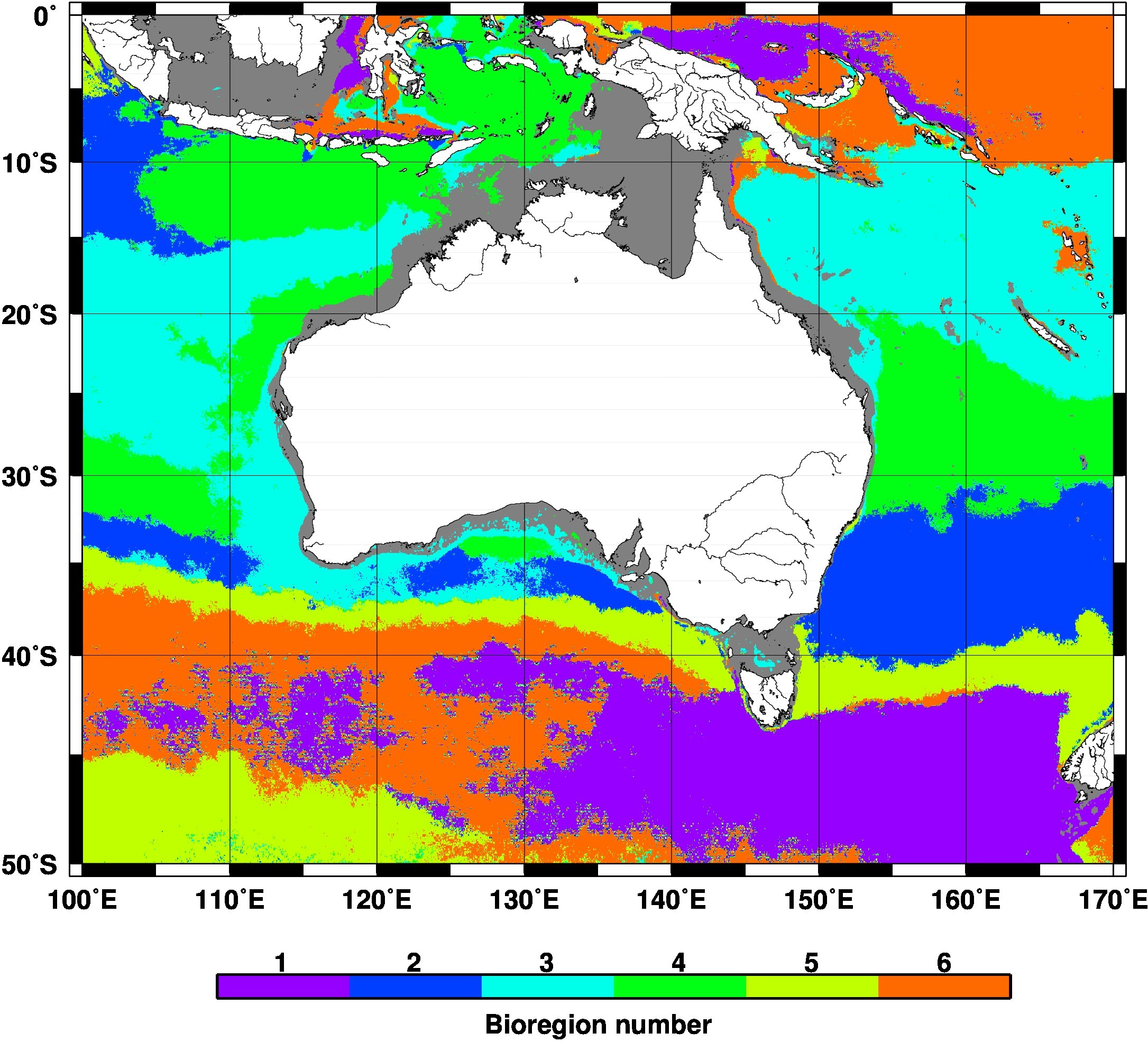
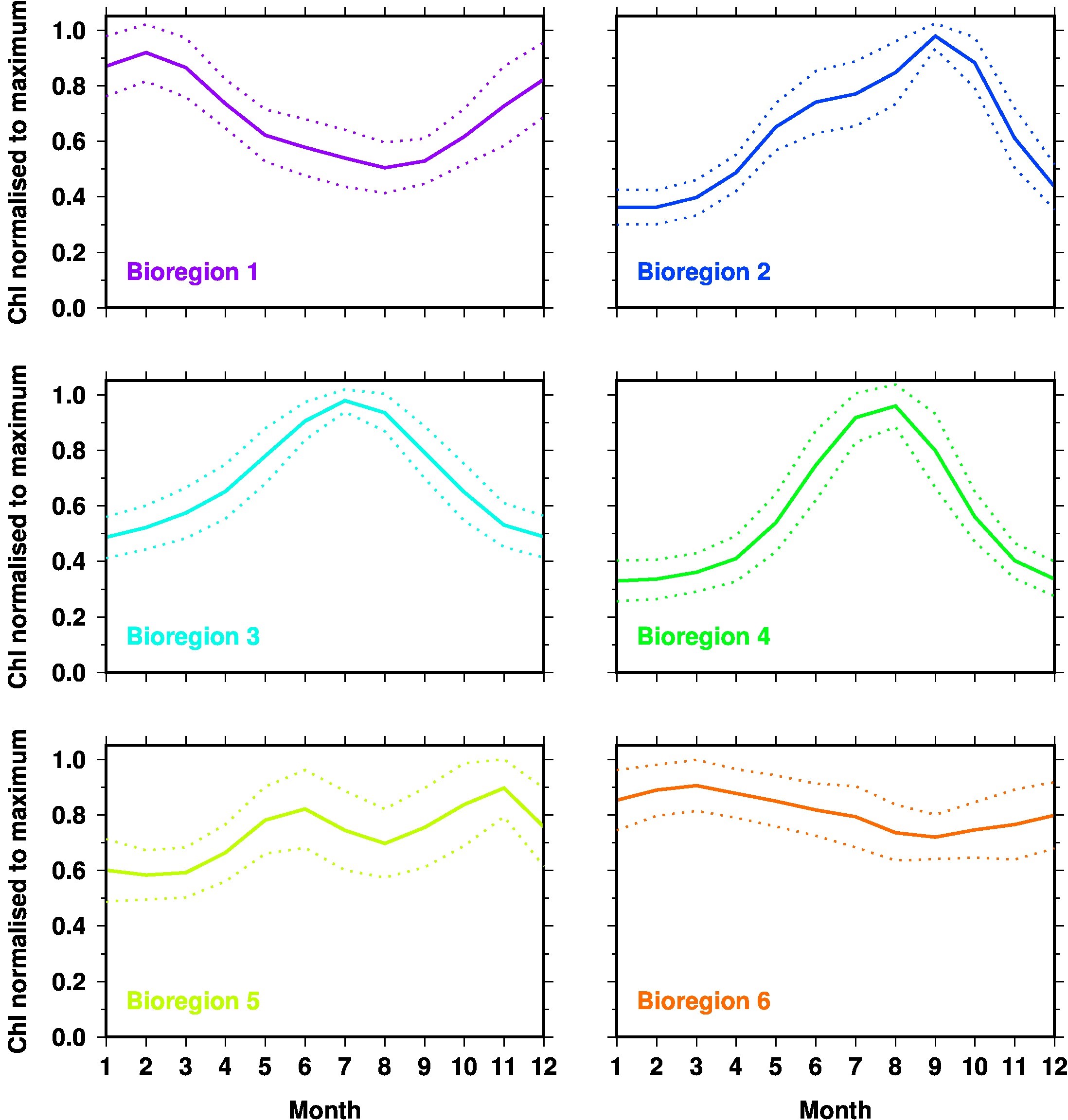
An analysis using satellite observations shows how phytoplankton amounts evolve along seasons around Australia, revealing broad areas of distinct seasonal patterns. These different phenology traits determine the functioning of the entire ecosystem, inasmuch as phytoplankton is the base of the entire oceanic foodweb.

Keywords

phytoplankton phenology, silhouette analysis, seasonal cycles

The seasons of phytoplankton around Australia

The study of naturally recurring events is known as “phenology” and has been largely developed and used in terrestrial ecosystem studies. Such events can be, for instance, the onset and duration of the spring growing season. Similar studies are now carried out for ocean ecosystems, with a particular emphasis on phytoplankton, which is the base of the marine foodweb and an important component of the marine carbon cycle. Here we characterise regional patterns of phytoplankton seasonal cycles, which is crucial to understanding relationships between climate (environment) forcing and marine ecosystems.

Our analysis used sixteen years (2003-2018) of satellite ocean colour observations from the NASA Aqua-MODIS sensor. Individual satellite images were processed using the SeaDAS software and applying the OCI chlorophyll algorithm (Hu, Lee, & Franz, 2012). Images were combined spatially and temporally into 4-km monthly composite maps of the chlorophyll concentration, further aggregated into twelve climatological monthly composite maps. A k-means based cluster analysis (D'Ortenzio & Ribera d'Alcalà, 2009) was then applied at each of the 4-km grid cell of these monthly climatological chlorophyll maps, after the data in each of these cells were normalised by their maximum. This technique groups pixels with similar seasonal cycles, without being overly influenced by the dominant signal from changes of the chlorophyll concentration. The optimal number of clusters was determined through a “silhouette” analysis (Rousseeuw, 1987). The mean within each cluster is then computed and provides the typical seasonal cycle representative of the group. Resulting mapping reveals broad ocean areas – referred to here as bioregions – where seasonal changes in phytoplankton are similar. These bioregions are likely to have similar underlying physical mechanisms and ecosystem responses. Depths shallower than 100 m have been excluded from the analysis.

The cluster analysis suggested six bioregions (Figure 1), with each having a distinctive seasonal cycle (Figure 2). Overall, the bioregions follow latitudinal bands, except in the Leeuwin Current and in the northeast Indian Ocean. Mid-latitude areas show a single seasonal maximum in July or August (bioregions #3 and #4). When moving further south, two maxima appear, in June and September for region #2, and June and November for region #5, which essentially matches the subtropical convergence. Interestingly the same seasonal pattern (#5) also appears further south in the western part of the study region, and corresponds to the Antarctic convergence. The area in-between these two major features of the physical oceanography of the Southern Ocean is split into two distinct bioregions around a longitude of 135°E. West of this, the seasonality is weak with a maximum in March, whereas the maximum is in February and the seasonal amplitude larger east of 135°E. Region #2 is quasi-absent west of the Australian continent. Consequently, the Leeuwin Current flowing south along the west coast of Australia includes only two major bioregions (#3 and #4), while the East Australian current crosses regions #3, #4 and #2. As for low-latitude areas (<10°S), an area of essentially low seasonality extends east of Papua New Guinea, whereas the Banda Sea (between Indonesia and Papua New Guinea) is entirely assigned to region #4, with a strong seasonal cycle showing a maximum in August. This same pattern appears south of Java.

Interactions between physics and biology in the ocean are complex. To some extent, delineating bioregions based on a simple indicator such as the shape of the seasonal cycle, captures this complexity and allows us to summarise it graphically.

The phenology of phytoplankton and the importance to fisheries production is encapsulated in the match-mismatch hypothesis (Cushing, 1989). This hypothesis states that the degree of match and mismatch in the timing of fish larval abundance and the production of their food (both phytoplankton and zooplankton) explains much of the variability in recruitment of fish. Thus, if fish spawn and larvae emerge when phytoplankton (and zooplankton) are high, then there is a match in timing and there is higher likelihood of fish larval survival because of good feeding conditions. By contrast, if fish spawn and larvae emerge when phytoplankton (and zooplankton) are low, then there is a mismatch in timing and there is higher mortality of fish larvae because of starvation. Thus, knowing the seasonality of phytoplankton is key to understanding whether higher trophic levels can find sufficient food at the right time of the year. Although the climatology presented here cannot address interannual variability, the same analyses can be performed on shorter and successive time periods to identify changes in the spatial distributions of bioregions.

A practical application of defining bioregions is to guide oceanographic sampling. The significant effort that is put into sampling the ocean is inevitably limited with respect to its vastness. Therefore, when designing research voyages or planning for deployment of autonomous profiling floats, maps such as the one derived here can help avoid oversampling some areas while missing others, in view of optimising the use of our sampling capability. They could also help when delineating boundaries of marine parks or marine protected areas.

Cushing, D. H. (1989). A difference in structure between ecosystems in strongly stratified waters and in those that are only weakly stratified. Journal of Plankton Research, 11(1), 1-13.

D'Ortenzio, F., & Ribera d'Alcalà, M. (2009). On the trophic regimes of the Mediterranean Sea: a satellite analysis. Biogeosciences, 6(2), 139-148. doi:10.5194/bg-6-139-2009

Hu, C., Lee, Z., & Franz, B. (2012). Chlorophyll a algorithms for oligotrophic oceans: A novel approach based on three-band reflectance difference Journal of Geophysical Research, Oceans, 117, C01011. doi:10.1029/2011jc007395

Rousseeuw, P. J. (1987). Silhouettes: A graphical aid to the interpretation and validation of cluster analysis. Journal of Computational and Applied Mathematics, 20, 53-65. doi:10.1016/0377-0427(87)90125-7

Figure 1

The 6 “bioregions” determined from the phenology of phytoplankton. The average normalised seasonal cycles are shown in Figure 2 (same colour coding). Shallow waters (depth <100m) where the satellite chlorophyll is less reliable have been excluded from the analysis and appear white on this map.

Figure 2

Mean normalised seasonal cycles for the 6 “bioregions” mapped in Figure 1 (same colour coding applies). The upper and lower curves in each panel indicate the standard deviation within the data cluster from which the average seasonal cycle (middle curve) was derived.

Download this Time Series Report

Citing this report: 

Antoine D, Mayot N, King E. (2020) The seasons of phytoplankton around Australia. In Richardson A.J, Eriksen R, Moltmann T, Hodgson-Johnston I, Wallis J.R. (Eds). State and Trends of Australia’s Ocean Report. doi: 10.26198/5e16a91249e7c

doi: 10.26198/5e16a91249e7c

Access the Data

Access the data that contributes to this time-series by clicking the icons below

06f. National Reference stations-02

Satellite Remote Sensing

Citing the Report

Richardson A.J, Eriksen R, Moltmann T, Hodgson-Johnston I, Wallis J.R. (2020). State and Trends of Australia’s Ocean Report, Integrated Marine Observing System (IMOS).

IMOS_logo-stacked-reversed-01

The State and Trends of Australia's Ocean Report was supported by IMOS. IMOS gratefully acknowledges the additional support provided by the Commonwealth Scientific and Industrial Research Organisation (CSIRO).

The State and Trends of Australia's Ocean website is maintained by IMOS.


NCRIS-PROVIDER-REV

Australia’s Integrated Marine Observing System (IMOS) is enabled by the National Collaborative Research Infrastructure Strategy (NCRIS). It is operated by a consortium of institutions as an unincorporated joint venture, with the University of Tasmania as Lead Agent.

Disclaimer:

You accept all risks and responsibility for losses, damages, costs and other consequences resulting directly or indirectly from using this site and any information or material available from it. While the Integrated Marine Observing System (IMOS) has taken reasonable steps to ensure that the information on this website and related publication is correct, it provides no warranty or guarantee that information provided by the authors is accurate, complete or up-to-date. IMOS does not accept any responsibility or liability for any actions taken as a result of, or in reliance on, information on its website or publication. Users should check with the originating authors to confirm the accuracy of the information before taking any action in reliance on that information.

If you believe any information on this website or in the related publication is inaccurate, out of date or misleading, please bring it to our attention by contacting the authors directly or emailing us at IMOS@imos.org.au


Images and Information:

All information on this website remains the property of those who authored it. All images on this website are licensed through Adobe Stock, Shutterstock, or have permission from the original owner.