Biological Time Series - Productivity

2.1

Spatial and seasonal trends in Chlorophyll a

Contributors

Peter Thompson1

David Antoine2

Edward King1

1 CSIRO Oceans and Atmosphere, Hobart, TAS, Australia
2 Remote Sensing and Satellite Research Group, School of Earth and Planetary Sciences, Curtin University, Perth, WA, Australi

Key Information

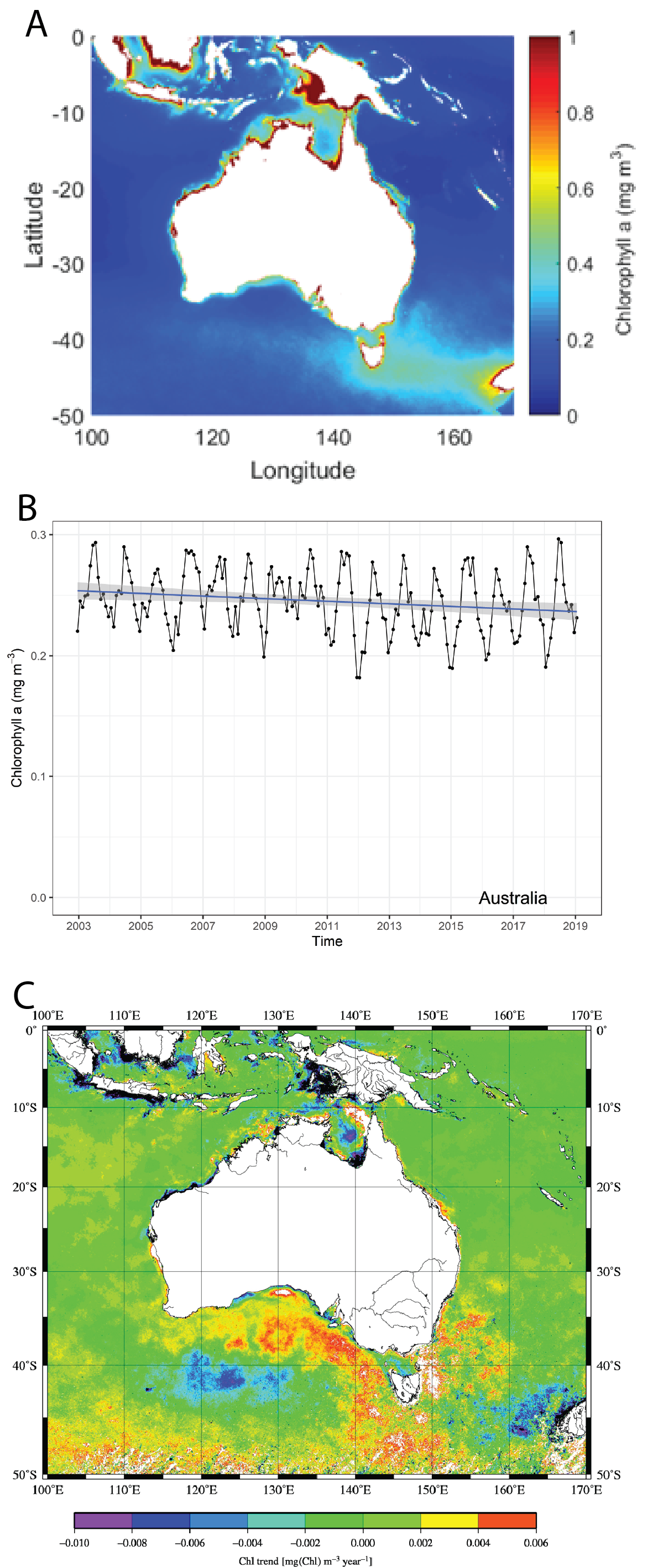
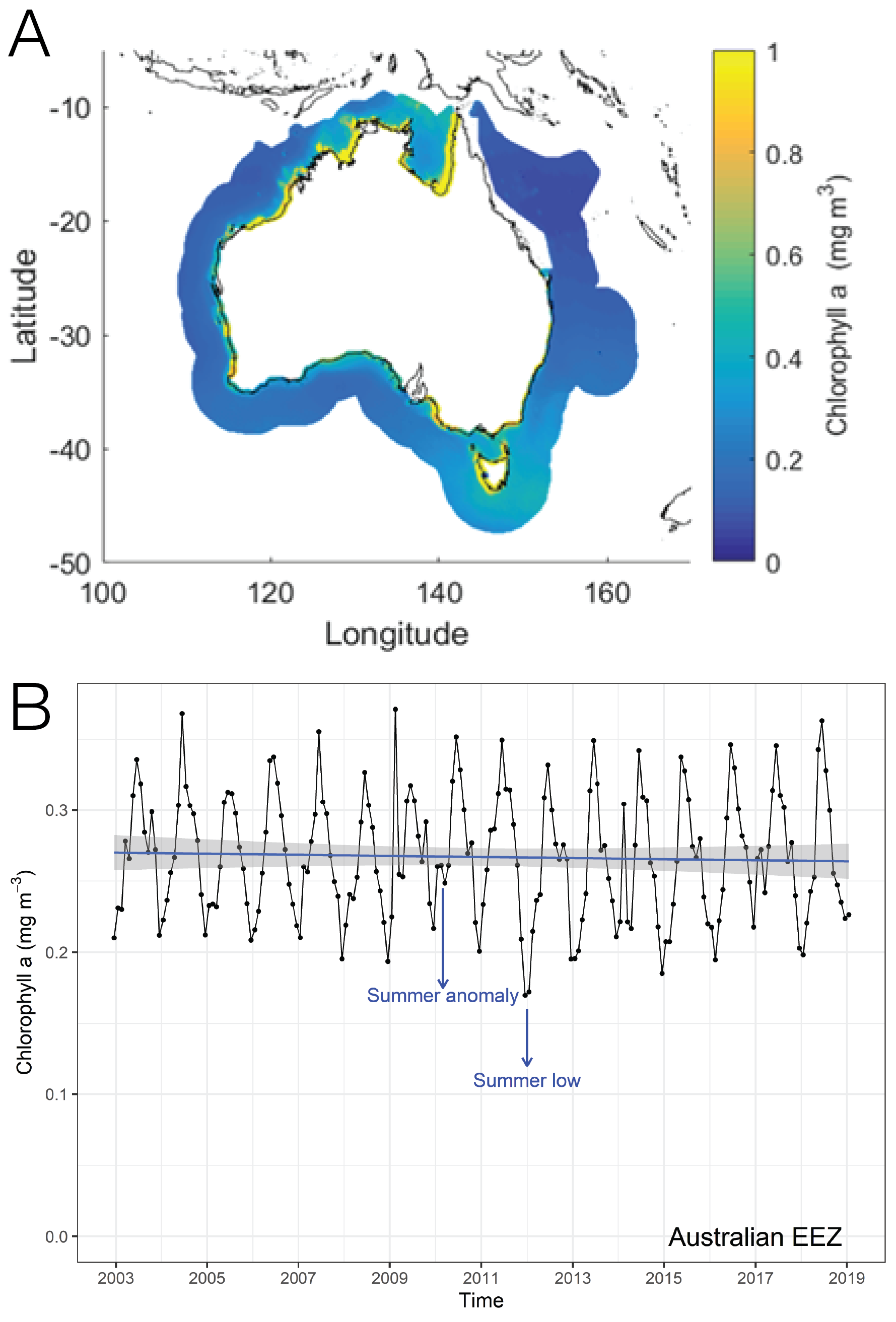
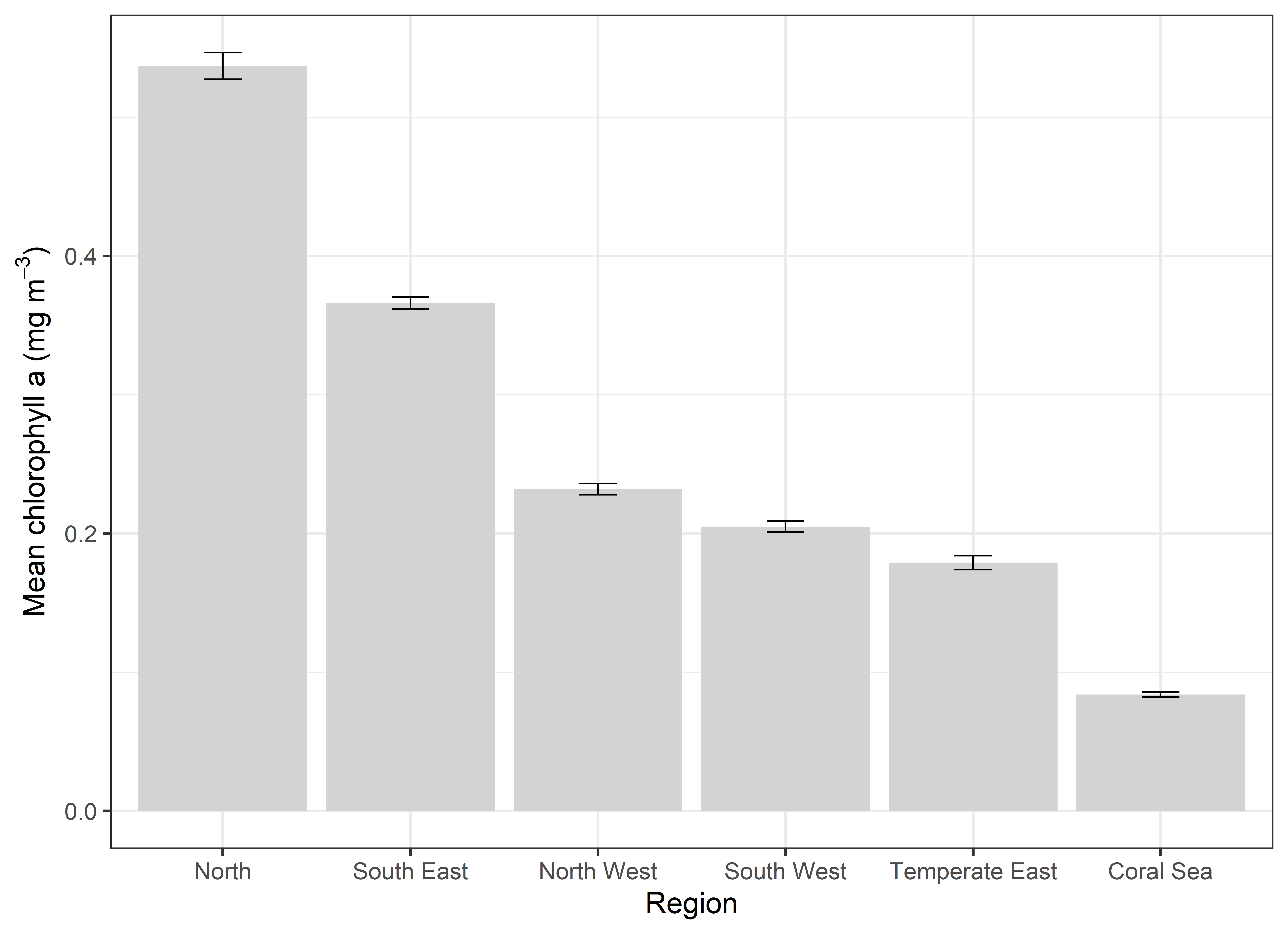
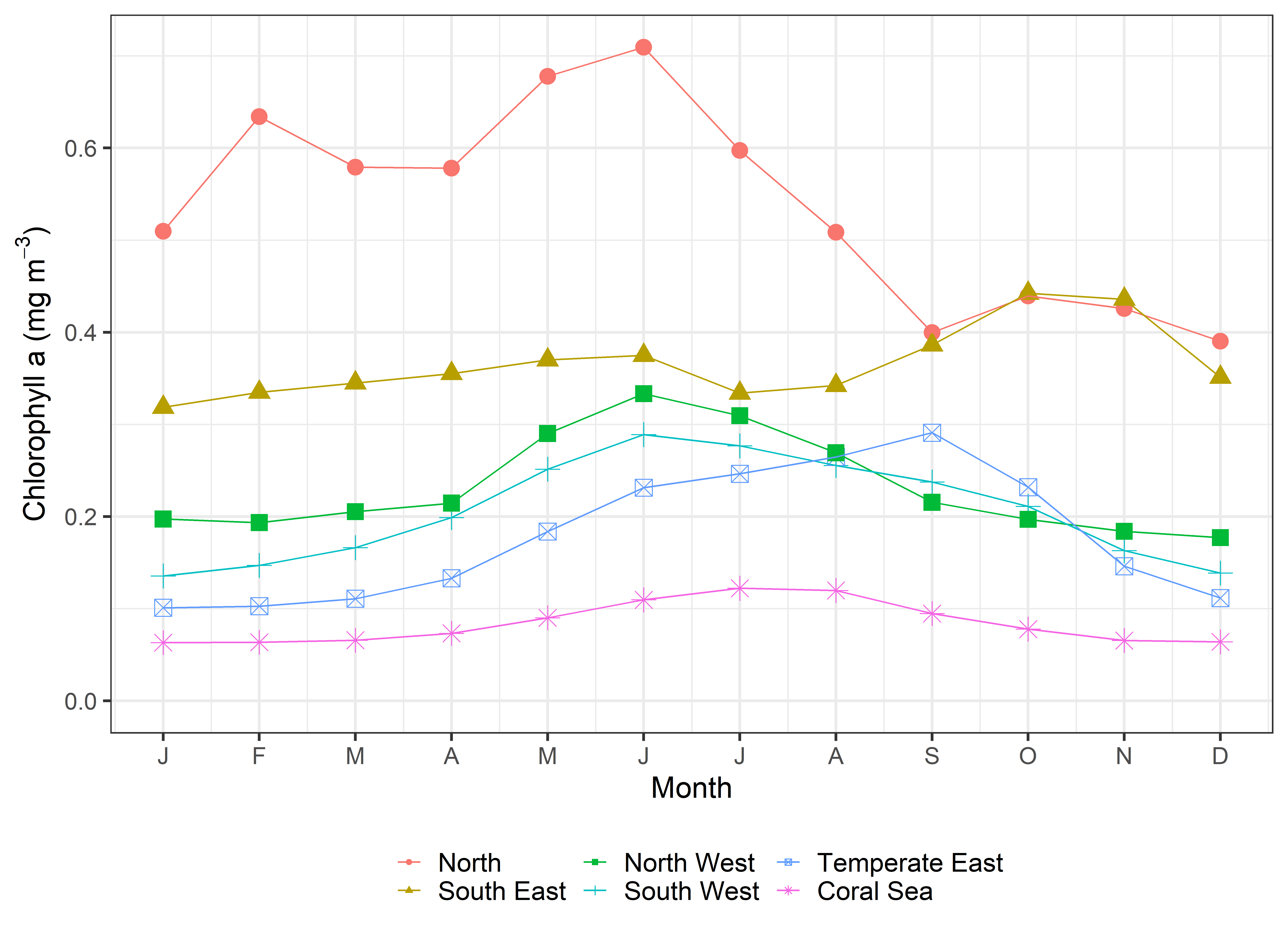
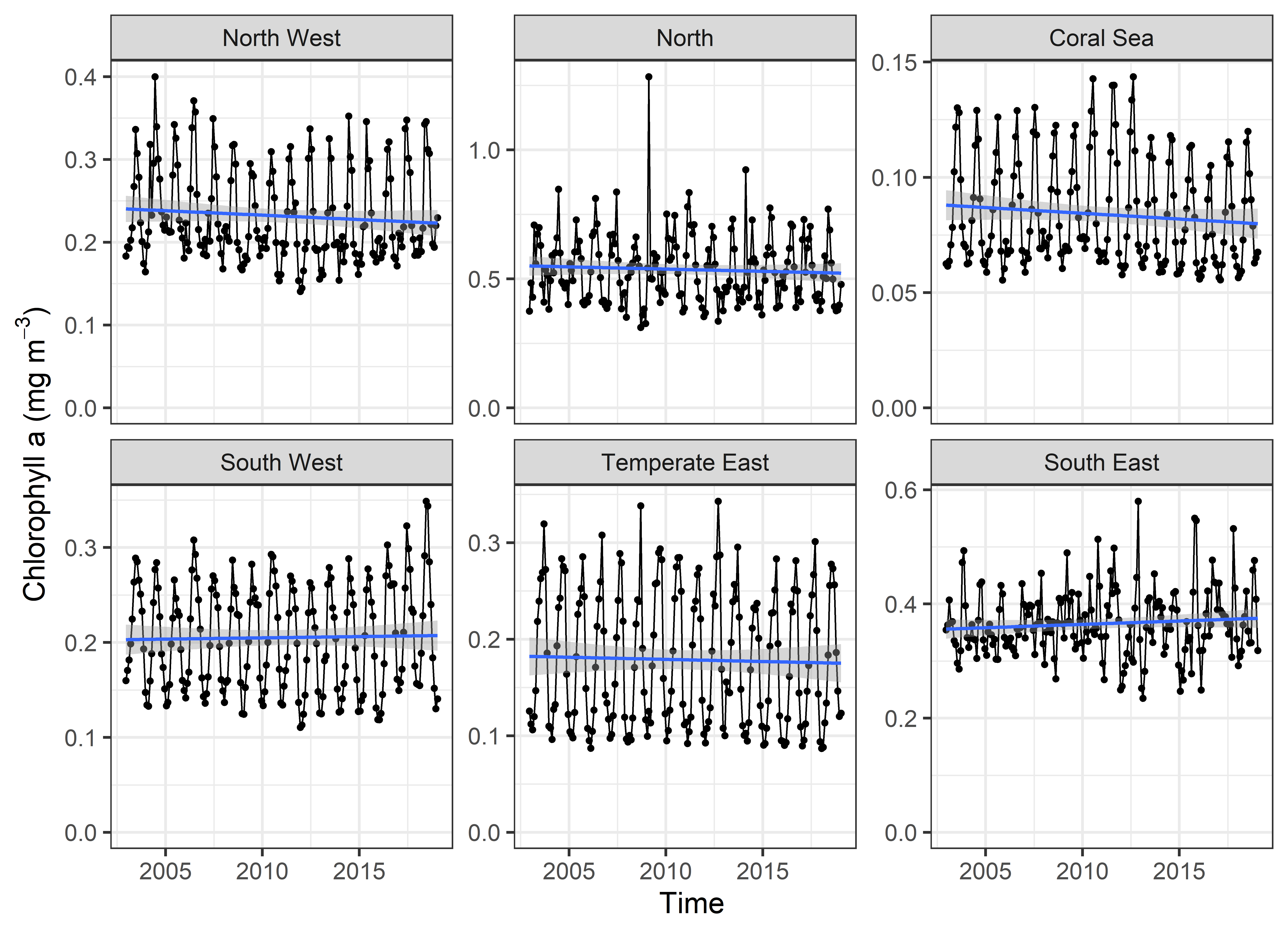
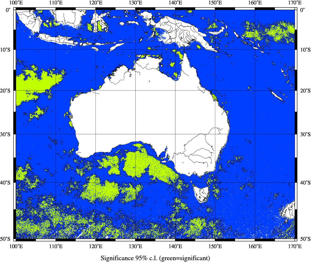
The concentration of chlorophyll a, a measure of phytoplankton biomass has seen an overall decline by 8% in Australian waters over the past 17 years. Despite this general marked decrease, large parts of the ocean south and southeast of Australia and the coastal zone along the east coast of Australia have seen significant increases in chlorophyll a concentration. Declines in chlorophyll a close to shore along the North West shelf and throughout the Great Australian Bight may significantly impact these coastal ecosystems and the fisheries they support.

Keywords

phytoplankton biomass, phytoplankton pigments

Spatial and seasonal trends in Chlorophyll a

Chlorophyll a is a pigment present in all photosynthetic phytoplankton species. The amount of chlorophyll a in water is internationally recognized as a simple but worthwhile measure of phytoplankton biomass. Chlorophyll enables phytoplankton to grow by capturing energy from the sun, thus earning phytoplankton the name “grass of the sea”. Without phytoplankton there would be almost no other life in the ocean – they provide oxygen, food for higher trophic levels, are important in carbon sequestration as they sink into the deep ocean and, therefore, are of great ecological significance (Sournia, 1978).

Chlorophyll a can be monitored relatively easily, but the use of satellites to measure chlorophyll a has revolutionized our ability to observe the spatial and temporal dynamics, especially large scales. These dynamics include seasonal patterns of phytoplankton abundance, climate cycles and any longer-term changes. Trends in chlorophyll a tend to reflect changes in the ocean’s physical and chemical dynamics as temperature plus light and nutrient availability are the primary determinants of phytoplankton growth. Temperature, light and nutrient concentrations have a range of natural cycles that drive most of the temporal variation in phytoplankton. This means that any longer-term climate-driven trends can be difficult to detect without a sufficiently long time series of measurements to apportion phytoplankton variation to the right driver.  

Phytoplankton pigments are a major source of colour in the world’s oceans and satellite technology has made it possible to obtain global estimates of this colour many times a year. The temporal and spatial sampling achieved by satellites produces a marvellous global estimate of phytoplankton biomass using well established empirical relationships. Research continues to reduce the small errors associated with variation in absorption and backscattering properties of phytoplankton and effects of coloured-dissolved organic matter and minerals (Dierssen, 2010).

Here we have used sixteen years of satellite data (2003-2018) from the MODerate resolution Imaging Spectroradiometer (Aqua-MODIS) sensor that estimates the near-surface concentration of chlorophyll a using an empirical relationship derived from in situ measurements of chlorophyll a and blue-to-green band ratios of in situ remote sensing reflectances. Full details can be found at https://modis.gsfc.nasa.gov/data/dataprod/chlor_a.php.

Satellite data were processed using the SeaDAS software with the OCI chlorophyll algorithm (Hu, Lee, & Franz, 2012). Data were analysed to give monthly composite maps of the chlorophyll a concentration. Linear temporal trends were extracted across a range of spatial scales from 4 km2 to the Australian region (50°S to equator, 100°E to 170°E), including analysis of the de-trended time series (the time series from which the mean seasonal cycle was removed).

Chlorophyll a within the Australian region

The mean chlorophyll a concentration in surface waters across the Australian region between the beginning of 2003 and the end of 2018 was 0.25 mg. m-3 (Figure 1a). This is a low concentration typical of healthy tropical and subtropical oceanic waters. Areas of markedly higher chlorophyll a include the coastal zone around Australia, seas between Australia and its northern neighbours, and waters between Tasmania and New Zealand.

The mean monthly chlorophyll a concentration varied seasonally and inter-annually (Figure 1b). There was, however, a significant (P<0.006) negative trend across the entire region over the period from 2003-2019 (Figure 1b), with the Chlorophyll a concentration declining ~8%. By contrast, there were large parts of the ocean south and southeast of Australia, and in the coastal zone along the eastern seaboard plus smaller patches throughout the shallow seas north of Australia there were significant gains in Chlorophyll a. (Figure 1c). Within the region the most significant (Figure S1) downward trends in Chlorophyll a were found between 120 and 130°E near 40°S, near the centre of the Gulf of Carpentaria and nearshore in two regions; parts of the North West Shelf and throughout much of the Great Australian Bight.

Chlorophyll a within the Australian EEZ

Within Australia’s continental EEZ the mean chlorophyll a concentration was 0.26 mg m-3 (Figure 2a). Chlorophyll a tended to be low in the tropical and subtropical oceanic regions; greater in the coastal zone, the shallow seas between Australia and its northern neighbours and around Tasmania.

As with the broader regional trend the overall EEZ has declined significantly in chlorophyll a (P<0.006) over the period from 2003 to 2019. The rate of decline was similar at ~8% over 16 years. The inter-annual variation shows the summer of 2011-12 was much lower in chlorophyll a than the summer of 2009-10 (see grey circles Figure 2b).

Chlorophyll a within the Australian bioregions

Australia has six marine bioregions around the continent plus several around islands such as Christmas, Cocos, Lord Howe, Macquarie and another along the Antarctic coast. In this report we assess the six bioregions around the continent (Figure 3a). They showed distinct differences in the mean state and trends for chlorophyll a, net primary production and turbidity.

All of the six bioregions have distinctly different (p<0.05) mean chlorophyll a concentrations (Figure 3b). The North bioregion has more than 6 times the mean chlorophyll a of the nearby Coral Sea (Table 1). The second greatest mean chlorophyll a is found in the southeast, in waters around Tasmania.  All bioregions showed some seasonal variability in chlorophyll a concentration, with the largest variability seen in the North bioregion where chlorophyll a peaked at 0.7 mg m-3 in July (Figure 4). The Coral Sea and both west coast bioregions (NW and SW) tended to reach peak chlorophyll a concentrations during winter. Both the Temperate East and the Southeast bioregions experienced spring blooms of phytoplankton. The Temperate East phytoplankton bloom reached peak biomass in September and the Southeast spring bloom peaked in October.

State and trends in chlorophyll a were assessed for each of the six bioregions (Figure 5). Mean values for each bioregion are all different (Table 1) and so are the trends (Table 2). There were no statistically significant positive trends in any bioregion. The Coral Sea, Temperate East and Northwest Bioregions all showed significant declines from 2002-2019.

The phytoplankton biomass around Australia is relatively low; a situation typical of most tropical and subtropical waters. Unlike most continents, Australia does not have large-scale upwelling along its west coast as it is supressed by the southward-flowing Leeuwin Current.

The North, Northwest, Southwest and Coral Sea all experienced greatest phytoplankton biomass in winter. By contrast, the Temperate East and Southeast regions show classic spring blooms during September or October. These periods of high phytoplankton biomass provide periods of peak food availability for zooplankton and are often the most important period for larval fish recruitment. The capacity for our marine ecosystems to sustain our existing biodiversity is dependent upon both the amount of phytoplankton present and the timing of the greatest biomass.  

Although the spatial patterns of change in Chlorophyll a are patchy from 2002-2019, the rate of change averaged over the region, the continental EEZ, and within 3 of the 6 bioregions was significantly negative. If the overall rate of decline is sustained at 0.5% per year, it will eventually cause a dramatic impact on the region’s marine ecology and is very likely to cause a reduction in many regional fish stocks. Declines in Chlorophyll a close to shore along the North West Shelf and throughout much of the Great Australian Bight are of considerable concern given the potential impacts on our coastal ecosystems. A longer time series and more in-situ monitoring should reveal whether this decline is caused by a climate cycle or is likely to persist if the planet continues to warm.  

Dierssen, H. M. (2010). Perspectives on empirical approaches for ocean color remote sensing of chlorophyll in a changing climate. Proceedings of the National Academy of Sciences of the United States of America, 107(40), 17073-17078. doi:10.1073/pnas.0913800107

Hu, C., Lee, Z., & Franz, B. (2012). Chlorophyll a algorithms for oligotrophic oceans: A novel approach based on three-band reflectance difference Journal of Geophysical Research, Oceans, 117, C01011. doi:10.1029/2011jc007395

Sournia, A. (1978). Phytoplankton manual. Retrieved from Paris

Figure 1

a) The mean Chlorophyll a (mg. m-3) across the Australian region (50°S to equator, 100°E to 170°E) from 2003 to 2019. b) mean monthly Chlorophyll a (mg. m-3) with a linear regression fitted showing trend at the same spatial scale. c) Trends in Chlorophyll a (mg. m-3 y-1) for each 4 km2 across the entire Australian region (50°S to equator, 100°E to 170°E) from 2003 to 2019.

Figure 2

a) The mean Chlorophyll a (mg. m-3) within the Australian Economic Exclusion Zone (EEZ) from 2003-2019 (the EEZ extends 200 nautical miles from the territorial sea baseline). b) mean monthly EEZ chlorophyll a fitted with a linear regression showing the long-term trend. Some anomalous summer months are circled. They demonstrate the interannual variability associated with climate cycles such as ENSO.

Figure 3

The mean Chlorophyll a (mg m-3) within each bioregion, from 2003 to 2019.

Figure 4

Monthly mean concentrations of Chlorophyll a (mg. m-3) within each of Australia’s six bioregions from 2003 -2019.

Figure 5

Mean monthly chlorophyll a concentrations (mg. m-3) for the six Australian bioregions from 2003 to 2019 including a linear regression showing the trend for each bioregion.

Figure S1

The statistical significance of the trends shown in Figure 1c (Student test, 95% confidence level).

Table 1

Mean Chlorophyll a (mg m-3) within each of Australia’s six bioregions from 2003 -2019.

Table 2

Assessment of linear trends for seasonally corrected (the average monthly mean is subtracted from each monthly value) chlorophyll a concentrations in 6 Australian bioregions over the period 2003 to 2019.

Download this Time Series Report

Citing this report: 

Thompson P, Antoine D, King E. (2020) Spatial and seasonal trends in Chlorophyll a. In Richardson A.J, Eriksen R, Moltmann T, Hodgson-Johnston I, Wallis J.R. (Eds). State and Trends of Australia’s Ocean Report. doi: 10.26198/5e16a44a49e79

doi: 10.26198/5e16a44a49e79

Access the Data

Access the data that contributes to this time-series by clicking the icons below

06f. National Reference stations-02

Satellite Remote Sensing

Citing the Report

Richardson A.J, Eriksen R, Moltmann T, Hodgson-Johnston I, Wallis J.R. (2020). State and Trends of Australia’s Ocean Report, Integrated Marine Observing System (IMOS).

IMOS_logo-stacked-reversed-01

The State and Trends of Australia's Ocean Report was supported by IMOS. IMOS gratefully acknowledges the additional support provided by the Commonwealth Scientific and Industrial Research Organisation (CSIRO).

The State and Trends of Australia's Ocean website is maintained by IMOS.


NCRIS-PROVIDER-REV

Australia’s Integrated Marine Observing System (IMOS) is enabled by the National Collaborative Research Infrastructure Strategy (NCRIS). It is operated by a consortium of institutions as an unincorporated joint venture, with the University of Tasmania as Lead Agent.

Disclaimer:

You accept all risks and responsibility for losses, damages, costs and other consequences resulting directly or indirectly from using this site and any information or material available from it. While the Integrated Marine Observing System (IMOS) has taken reasonable steps to ensure that the information on this website and related publication is correct, it provides no warranty or guarantee that information provided by the authors is accurate, complete or up-to-date. IMOS does not accept any responsibility or liability for any actions taken as a result of, or in reliance on, information on its website or publication. Users should check with the originating authors to confirm the accuracy of the information before taking any action in reliance on that information.

If you believe any information on this website or in the related publication is inaccurate, out of date or misleading, please bring it to our attention by contacting the authors directly or emailing us at IMOS@imos.org.au


Images and Information:

All information on this website remains the property of those who authored it. All images on this website are licensed through Adobe Stock, Shutterstock, or have permission from the original owner.